When images are taken with a VK-X1000 series microscope you cannot measure the distance between separate images in the Keyence Multifile Analyzer, or any other software that Keyence offers. Measurements can only be performed within the images themselves.
With the standard tools you can stitch together an area to get one large image, but there is a limitation to the number of images that can be stitched together (100 or 560 depending on resolution) and this would be a time consuming process. A 30 second acquisition per image for 100 images would take 50 minutes, and the area being collected would only cover a 32 x 24 mm area with an x5 magnification.
With a 200mm wafer these limitations can cause the process to be so time consuming it is not worth doing.
Utilizing the XpansionUI and an Excel spreadsheet we can utilize the high resolution encoders of the positioning system to register each image in stage space. Then with the Multifile Analyzer we can frame each area and get the exact global coordinates of a feature. This would be propagated to each image with the Keyence MultiFileAnalyzers batch analysis function. After these measurements are exported to excel the stage coordinates for each image can be imported from the teach file used to create the images and the image positions and stage coordinates will be used to calculate the exact location of these features in tool coordinates.
The accuracy of this method is dependent on the stage accuracy and the microscopes accuracy.
The stage accuracy is determined by stage type. Peak Metrology uses Aerotech stages, which are designed for accuracy, repeatability and durability. With Aerotechs extensive catalog of stages Peak Metrology selects stages that will deliver the best value for the application. Typical Aerotech ballscrew and linear motor stages have an accuracy of +/-10um over 300mm of travel, uncalibrated.
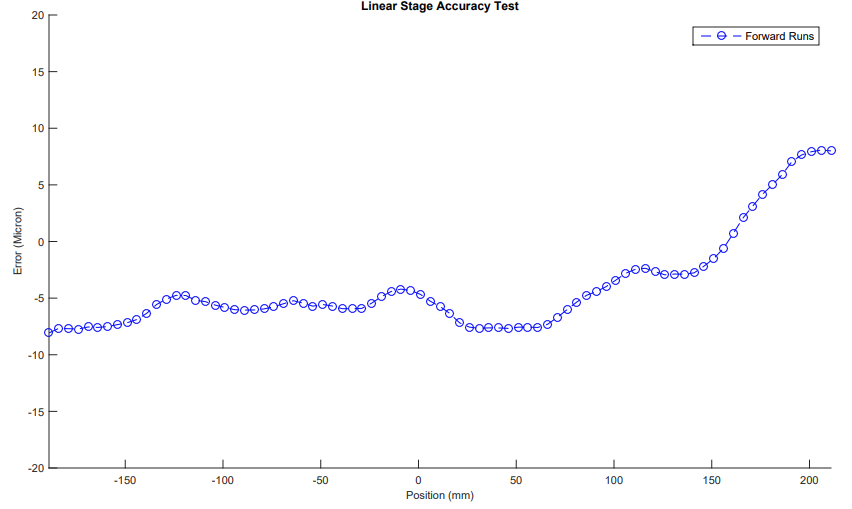
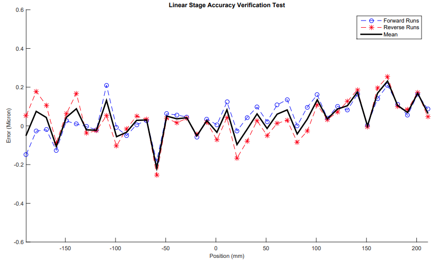
Since the XpansionUI also utilizes the Aerotech Automation1 Motion Controller we can calibrate the stages to compensate for these errors in motion. This brings a 300mm stages accuracy down to +/-2.5um for a ballscrew stage and +/-1.5um for a linear motor stage. This calibration increases performance by at least 400% and is performed on all LF-X systems. This is not done on any of the LF-B systems that are controlled by the Keyence controller, since they use open loop stepper motors and have no way to implement a calibration table.
The microscope also has an impact on accuracy. The Keyence VK-X1100 is accurate to within +/-2% of the measured value. This measured value is dependent on the lens being used and its magnification. The images are all taken with 1024×768 pixels. A low magnification lens will have a larger pixel size and thus will give us more variability in our measurements with the MultiFileAnalyzer.
Another impact on accuracy with the stitching method over a large area is a loss of resolution. When the images are stitched together the pixel count decreases. A standard resolution image is taken with a 1024×768 pixel count. When stitching together the maximum image count of 560 this resolution will be compressed. A fully stitched image of that size pixel count on a 56×10 image grid will be reduced to 12563×1676 pixels. If there was no compression we would have a pixel count of 50304×6816 when accounting for the 12.5% overlap when stitching. This compression results in images of less clarity.
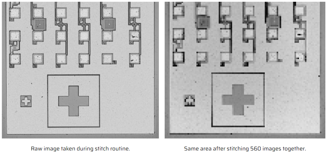
The loss of resolution will impact your measurements, as the edges are not as clear and the image is much blurrier, some features are completely missing between these two versions of the same image.
The VK-X1100 uses a revolver to change lenses. When the turret rotates to a new lens the center of the field of view shifts slightly. The Turret Calibration section of the Settings in the XpansionUI can minimize this effect, but the non-repeatable portion of this rotation will cause some shifts in your measurements. For the most accurate results use the same lens throughout this process.
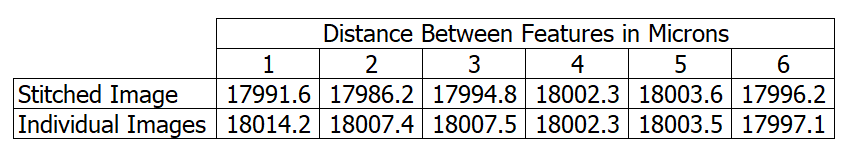
To show the accuracy of this process we measured distances on a large stitched image to a series of static images taken separately. The large stitched area, of 560 images, took over 9 hours to complete. The five images taken at the points of interest took less than five minutes. Since the VK-X can only stitch a maximum of 560 images together this limits the max area you can stitch together to measure. With a high magnification lens, say an x50 lens, this only allows for an area around 30 x 1.5 mm at best. This is a small area when looking at features on a 200mm wafer or another large part, not to mention the time required to take all of those images will be measured in hours, not minutes.

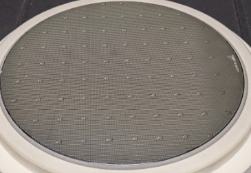
The image to the left shows the 200mm diameter wafer that we measured on. The box shows an estimate of the maximum area we can stitch using a x5 lens, around 135 x 18mm. The circles represent the areas of interest within this stitched image. The triangles represent areas we could measure using the Image Registration teaching method. Higher magnification lenses will limit our max stitching area, but have no impact on the image registration to the global positions. In fact the higher magnification will allow for finer detailed images that can be more accurately measured.
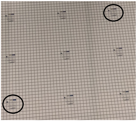
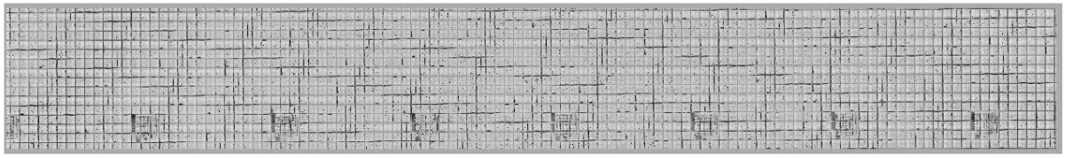
The above image is the fully stitched area of the 560 images taken. This image encompasses an area of 135 x 18mm over a 200mm diameter wafer. It took 8 hours and 54 minutes to create this image. The size of each pixel after the image is stitched is 10.7um squared. The raw image pixel size is 2.7um squared. We will look at 7 specific locations inside of this image, and measure the distances between these features. Then we will compare the raw files that compose the stitched area, which took less than 7 minutes to take, and compare the distance values between features. Image subjectivity when picking our point of interest will give us some variability in the measurement.

Teaching Once – Measuring Many
Creating a teaching routine that can be used on multiple parts will automate your process. Teach files assume that you are always starting at the same point, so some kind of fiducial alignment will be required.
- Load part and align to your microscope and measurement plane.
- Create a teaching routine that will image each point of interest on your part.
- Execute the teaching routine which will save all of your results to the PC/network.
- Using an image analyzer find the center point of the image.
- Calculate the X and Y distance from the center point of the image to the far edge of the image. This distance creates a frame of reference for all features being measured in each image.
- Calculate the X distance from the X reference edges to the point of interest.
- Calculate the Y distance from the Y reference edges to the point of interest.
- Repeat steps 5 – 7 for all images taken. Hopefully your analysis package has a batch analysis to make this easier.
- Export all measurements to a spreadsheet.
- Import teaching locations for each image into the spreadsheet.
- Tie each teach points coordinates to the appropriate image.
- Subtract the X distance to the frame edge value from step 5 from the X Center point location from the teach file X value from step 11 and add the distance calculated in step 6.
- Subtract the Y distance to the frame edge value from step 5 from the X Center point location from the teach file Y value from step 11 and add the distance calculated in step 7.
- Repeat steps 12 and 13 for all points of interest and all images taken.
- The values calculated in steps 12 & 13 are the coordinates in stage space of the point of interest.
Calculate the distance between any two features via the formula: √(X1-X2)2+(Y1-Y2)2