The Field of View Problem
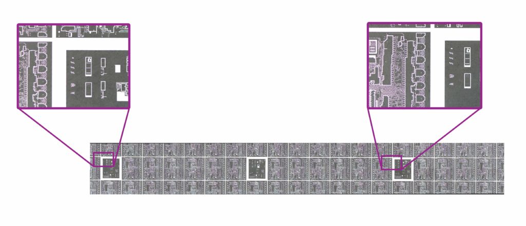
Microscopes are ideal for taking measurements at high magnification. They make measuring micro and nanoscale features simple. Specifically, measuring features within a microscope’s field of view is easy with off-the-shelf tools. However, when the features on the part being measured are not located within the microscope’s field of view it can quickly turn into a time-consuming measurement process. This is because most microscopy systems have to take multiple single field of view measurements and stitch them together in order to provide a larger field of view. This also leads to exceptionally large measurement file sizes. Many times we only care about measuring certain features across the larger surface. Why gather all the unnecessary data in between these individual features if we don’t need to?
The Solution
We can use positioning stage encoders to tell us where the microscope is globally across the measurement surface. Then, we can use the microscope’s individual field of view to image the features of interest. Relating the encoder feedback with the microscope’s field of view will provide the necessary tie between the local measurement and global part surface coordinates. Effectively, this turns a field of view limited microscope into a nanoscale capable Coordinate Measuring Machine (CMM).
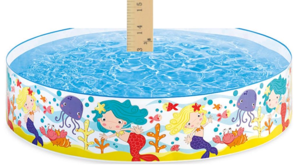
Here’s a simple example of how this principle works. When measuring the depth of a child’s pool, only two points are used on the ruler. One point is resting on the bottom of the pool and the second is the waterline on the ruler. The scale on the ruler relates the two points together. This is not unlike the encoder scale on a positioning stage. The waterline is akin to the measurement taken within a Microscope’s single field of view. Now, by using the ruler’s gradient markings showing just above the water we know the exact depth of the pool. And notably, we know the depth without needing to collect any data points between the bottom and top water surfaces.
Wait… there’s another limitation to keep in mind?
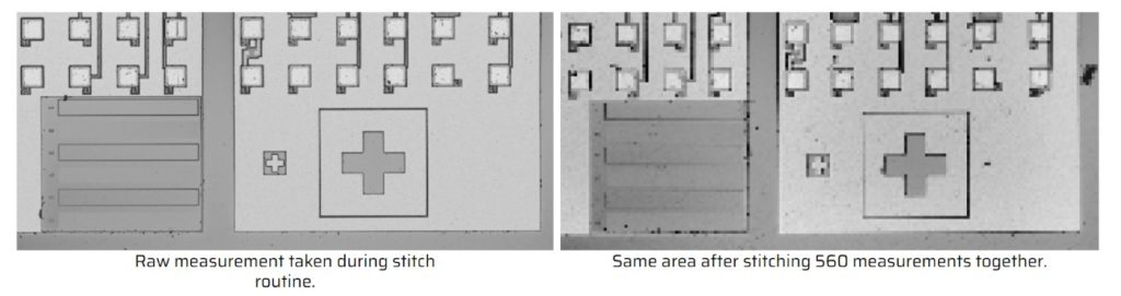
When the number of images in a stitched pattern increases there is often compression losses that lead to reduced resolution. This is a practical limit to how big the stitched image file size can get before it is too large to open easily. Therefore, reduced image count ensures each individual measurement is of the highest quality and not decimated by the stitching algorithm. The image below is an example of a stitched image losing its resolution due to decimation. The decimation is required to keep the file size manageable.
Implementing the solution
Implementing a way to reduce the image count necessary to take an image is a simple process once you have a positioning stage with encoder feedback in your microscopy setup.
- Load part onto stage and align it to the microscope’s coordinate frame.
- Use the stage to move to each feature of interest and capture measurement data using the microscope. Save the stage positions at each measurement location. Pro tip: A teaching routine (recipe file) can automate this process.
- Use the microscope’s analysis software to measure the feature relative to the center of the measurement’s field of view.
- Combine the individual field of view measurements with the global encoder measurements. This will produce global feature location measurements.
Faster More Accurate Outcomes
Each measurement on our microscope takes about 30 seconds to acquire. When features are too far apart we need to take many measurements in order to capture an overall area that includes all of the features at once. For an area size that requires 100 individual measurements, it takes us a minimum of 30 minutes to acquire and stitch all the individual measurement areas spanning multiple features.
Now let’s compare the above with our ability to use global encoder data to relate features together. With this process, we will cut the data acquisition time down by up to 95% by simply taking individual measurements at each feature location. Again, this is done by using the positioning system’s encoder scales to relate the dimensional information between the features that are far apart. Furthermore, since we reduced the image count we are able to remove stitching compression losses which can improve the resolution of each measurement by up to a factor of 25.
For more guidance and consultation on selecting the right positioning system reach out to us.